פרק 6 אקונומטריקה
בשביל זה אנחנו בעצם פה, לא?
נטען את החבילות הרלוונטיות
library(readstata13)    # Read Data Stored by stata13
library(stargazer)      # generate tables and regressions' output
library(sandwich)       # SE Clustering-robust adjustment
library(multcomp)       # Statistical tests
library(lmtest)         # Statistical tests

library(fixest)

library(data.table)
library(ggplot2)
6.1 אמידת רגרסיה
אמידת רגרסייה בשיטת הריבועים הפחותים מבוצעת ע”י שימוש בנוסחת lm.
- הפקודה מחזירה את האומדים למשתנים שהוכנסו לרגרסייה. על מנת לקבל מידע מפורט יותר, הכולל ס”ת, רמות מובהקות,
\(R^2\) וכו’ יש להשתמש בפקודה
summaryעל האובייקט. - ניתן לציין לפקודה שרוצים לאמוד את y באמצעות כל יתר המשתנים כך-
.~y. - אם מעוניינים להשתמש במודל ללא חותך יש להוסיף למשוואת האמידה את הביטוי
1-.
data(iris)

lm(Sepal.Length~Petal.Width+Sepal.Width,data=iris ) #רגרסיה עם חותך
##
## Call:
## lm(formula = Sepal.Length ~ Petal.Width + Sepal.Width, data = iris)
##
## Coefficients:
## (Intercept) Petal.Width Sepal.Width
## 3.4573 0.9721 0.3991lma<-lm(Sepal.Length~-1+Petal.Width+Sepal.Width,data=iris ) #רגרסיה עם חותך ששמרנו בתור אובייקט בשם lma
summary(lma)##
## Call:
## lm(formula = Sepal.Length ~ -1 + Petal.Width + Sepal.Width, data = iris)
##
## Residuals:
## Min 1Q Median 3Q Max
## -1.51065 -0.37958 0.01856 0.49083 1.65493
##
## Coefficients:
## Estimate Std. Error t value Pr(>|t|)
## Petal.Width 1.28202 0.05981 21.43 <2e-16 ***
## Sepal.Width 1.39229 0.02750 50.63 <2e-16 ***
## ---
## Signif. codes: 0 '***' 0.001 '**' 0.01 '*' 0.05 '.' 0.1 ' ' 1
##
## Residual standard error: 0.6116 on 148 degrees of freedom
## Multiple R-squared: 0.9894, Adjusted R-squared: 0.9893
## F-statistic: 6910 on 2 and 148 DF, p-value: < 2.2e-166.1.1 ייצוא טבלאות
דרך נוחה להציג מספר ספציפיקציות היא דרך חבילות
stargazer,modelsummary. חבילות אלה מאפשרות לייצא את טבלאות האמידה לקבצים בפורמטים שונים ובניהם,latex,html,doc.כיום, אני משתמש באופן כמעט בלעדי בחבילת
fixestכיוון שבאמצעותה אני יכול לבצע אמידות מסוג 2SLS, קלאסטרינג לסטיות התקן, ייצוא של טבלאות ללאטך, וגם כי היא מאד (מאד) מהירה (בדומה לפקודת reghdfe)כעת נייצא את טבלאת האמידה באמצעות
stargazerובהמשך נעשה זאת באמצעותetableששייכת לחבילתfixest
lma<-lm(Sepal.Length~-1+Petal.Width+Sepal.Width,data=iris ) # Same as earlier
lmb<-lm(Sepal.Length~Petal.Width+Sepal.Width,data=iris ) # Same as earlier

stargazer(lma,lmb,
type ='html',digits = 3,no.space=TRUE)| Dependent variable: | ||
| Sepal.Length | ||
| (1) | (2) | |
| Petal.Width | 1.282*** | 0.972*** |
| (0.060) | (0.052) | |
| Sepal.Width | 1.392*** | 0.399*** |
| (0.027) | (0.091) | |
| Constant | 3.457*** | |
| (0.309) | ||
| Observations | 150 | 150 |
| R2 | 0.989 | 0.707 |
| Adjusted R2 | 0.989 | 0.703 |
| Residual Std. Error | 0.612 (df = 148) | 0.451 (df = 147) |
| F Statistic | 6,909.605*** (df = 2; 148) | 177.556*** (df = 2; 147) |
| Note: | p<0.1; p<0.05; p<0.01 | |
6.1.2 שימוש בקטגוריות
אם רוצים להריץ רגרסיה שמתייחסת לערכים במשתנה מסויים כקטגוריאלים, ולהפוך כל ערך כזה למשתנה דמי, ניתן להשתמש להגדיר את המשתנה כ
factor
בדאטה עצמו, או להוסיף למשוואת הרגרסייה את המשתנה בתור פאקטור ע”י
factor(variable)
relevel
בסינטקס הבא:
relevel(df$var, var = “base”)
דוגמה בצ’אנק הבא
6.1.3 אינטרקציה
כאשר אומדים רגרסיה עם משתנה אינטרקציה, ניתן לחשוב על שני מקרי אפשרים, אם אנחנו רוצים לאמוד גם את המשתנים בנפרד ללא האינטרקציה, או אם אנחנו רוצים לאמוד את האינטרקציה בנפרד ללא המשתנים ממנה היא מורכבת.
כדי לאמוד את האינטרקציה לבדה (ללא המשתנים מהם היא מורכבת) נשתמש בסימן :,פעולה זו שקולה ל
#
בסטטה. כאשר נרצה לאמוד גם את המשתנים המרכיבים את האינטרקציה נשתמש ב
*
השקול ל
##
בסטטה.
data(iris)
iris$Species<-as.factor(iris$Species)
iris$Species<-relevel(iris$Species,"virginica")

lma<-lm(Sepal.Length~Petal.Width+Sepal.Width:Species,data=iris )
lmb<-lm(Sepal.Length~Petal.Width+Sepal.Width*Species,data=iris )

stargazer(lma,lmb,
type ='html',digits = 3,no.space=TRUE)| Dependent variable: | ||
| Sepal.Length | ||
| (1) | (2) | |
| Petal.Width | 0.390* | 0.351 |
| (0.210) | (0.213) | |
| Sepal.Width:Speciesvirginica | 0.855*** | |
| (0.165) | ||
| Sepal.Width | 0.741*** | |
| (0.217) | ||
| Speciessetosa | -1.043 | |
| (0.823) | ||
| Speciesversicolor | -0.192 | |
| (0.809) | ||
| Sepal.Width:Speciessetosa | 0.487*** | -0.073 |
| (0.096) | (0.268) | |
| Sepal.Width:Speciesversicolor | 0.782*** | -0.023 |
| (0.143) | (0.278) | |
| Constant | 3.249*** | 3.674*** |
| (0.332) | (0.596) | |
| Observations | 150 | 150 |
| R2 | 0.729 | 0.733 |
| Adjusted R2 | 0.722 | 0.721 |
| Residual Std. Error | 0.437 (df = 145) | 0.437 (df = 143) |
| F Statistic | 97.539*** (df = 4; 145) | 65.274*** (df = 6; 143) |
| Note: | p<0.1; p<0.05; p<0.01 | |
ניתן להשתמש בסוגריים כדי לבדל
x1<-rnorm(100)
x2<-runif(100)
x3<-sample(c(0,1),size = 100,replace = TRUE)
epsilon<-rnorm(100)
y<-(x1+x2+x1*x2)+(x1*x3+x2*x3+x1*x2*x3)+epsilon
# equ to y<-(x1+x2+x1*x2)*(1+X3)+epsilon

lm(y~(x1+x2+x1:x2)+(x1:x3+x2:x3+x1:x2:x3))  #שווה לאפס X3 במצב הבסיס
##
## Call:
## lm(formula = y ~ (x1 + x2 + x1:x2) + (x1:x3 + x2:x3 + x1:x2:x3))
##
## Coefficients:
## (Intercept) x1 x2 x1:x2 x1:x3
## 0.007668 0.542778 0.578435 2.011426 1.763858
## x2:x3 x1:x2:x3
## 1.354774 -0.699032lm(y~(x1*x2):factor(x3)) #Xעם ובלי משתנה 3##
## Call:
## lm(formula = y ~ (x1 * x2):factor(x3))
##
## Coefficients:
## (Intercept) x1:factor(x3)0 x1:factor(x3)1
## 0.007668 0.542778 2.306635
## x2:factor(x3)0 x2:factor(x3)1 x1:x2:factor(x3)0
## 0.578435 1.933208 2.011426
## x1:x2:factor(x3)1
## 1.312393lm(y~(x1+x2+factor(x3))^2) #לבד ואת כל האינטרקציות בזוגות של המשתנים##
## Call:
## lm(formula = y ~ (x1 + x2 + factor(x3))^2)
##
## Coefficients:
## (Intercept) x1 x2 factor(x3)1
## 0.1854 0.7436 0.3382 -0.2812
## x1:x2 x1:factor(x3)1 x2:factor(x3)1
## 1.6843 1.3966 1.71836.1.4 רגרסיות באמצעות FIXEST
המבנה של הנוסחה מעט שונה בחבילה הזו, והוא מהצורה הבאה
y~x|FE|IV
היתרון הוא שכאשר יש מספר רב של אפקטים קבועים
(FE)
החבילה הזו עובדת בצורה מהירה יותר משמעותית מחבילת
lm
שלעיתים אפילו לא תצליח לרוץ בגלל מגבלת זיכרון.
כעת נשחזר את התוצאות שהוצגו לעיל באמצעות פקודת
feols
מחבילת
fixest
fixest1<-feols(Sepal.Length~Petal.Width+Sepal.Width+Species,se="standard",data=iris )
fixest2<-feols(Sepal.Length~Petal.Width+Sepal.Width|Species,se="standard",data=iris )

etable(fixest1,fixest2,
       #file = "fixest.tex",replace=TRUE # Uncomment if you wish to save the latex table
       title = "This is a test",
       label="reg_results",
       tex = TRUE,
       style.tex = style.tex("aer",tabular="*"))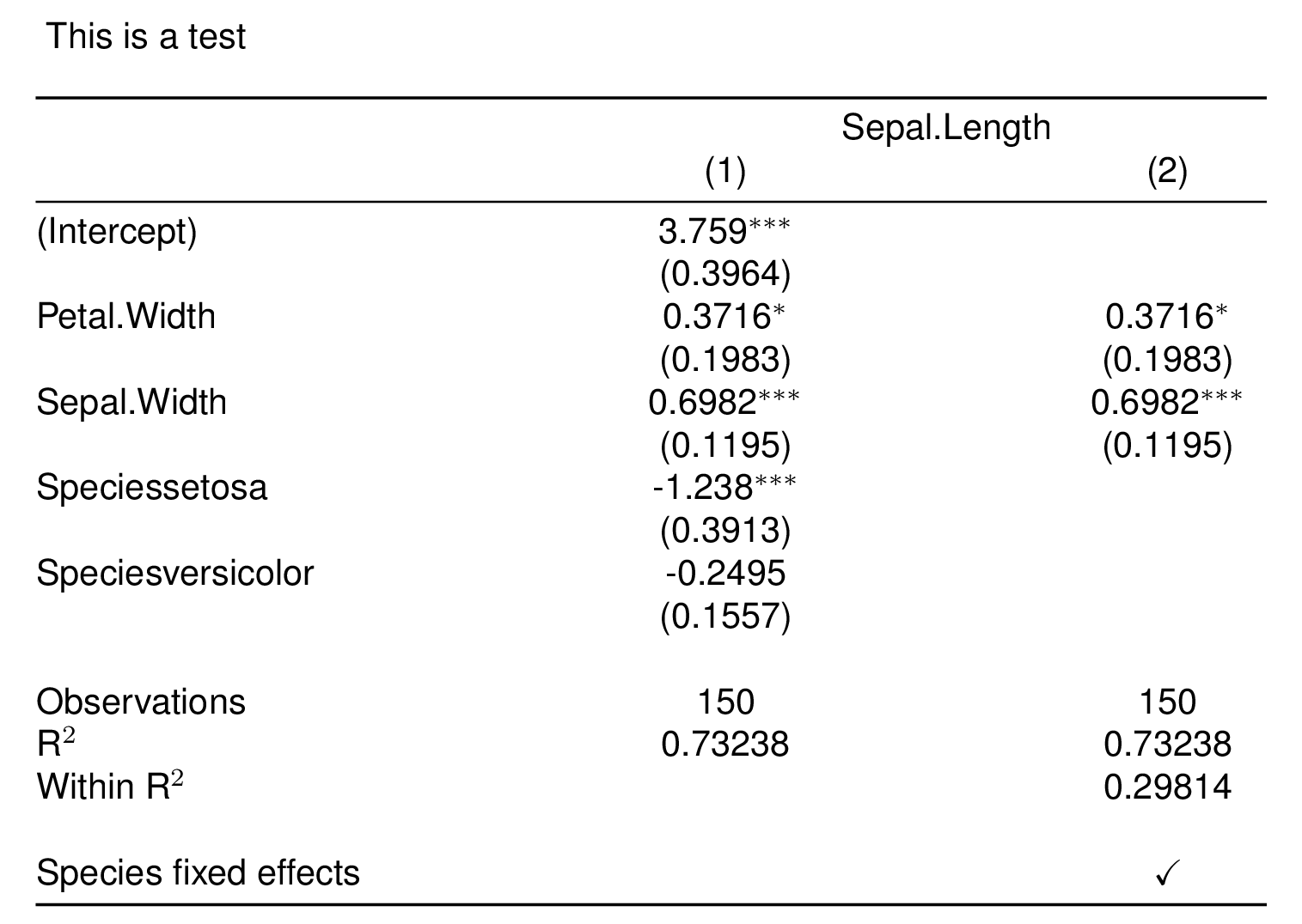
6.1.5 אינטרקציות ב-Fixest
כפי שראינו הנוסחה שמכניסים לאמידה היא מהצורה הבאה
y~x|FE
אם אנחנו רוצים להכניס אינטרקציות בחלק של המשתנים המסבירים
x
אנחנו יכולים להשתמש בסימונים הרגילים שראינו ב-
6.1.3
אם אנחנו רוצים להכניס אינטרקציות על ה
fixed effects
נשתמש באופרטור
^
החבילה מאפשרת לבצע leads-and-lags בצורה נוחה ופשוטה ע”י שימוש בפקודת אינטרקציה ייעודית, הפקודה היא מהצורה:
i(factor_var = time,var = treat,ref = -1)
6.2 תיקוני רובסט/קלאסטרינג
בעבר ביצעתי את התיקונים בצורה ידנית על ידי שינוי של מטריצת השונויות בעזרת החבילות
sandwich
ו-
lmtest.
לאחרונה גיליתי את שתי החבילות המעולות
lfe
ו-
fixest
שדומות לפקודת
reghdfe
של סטטה, ובנוסף, מבצעות את תיקוני ס”ת בצורה אוטומטית.
תיקוני סטיות תקן וקלאסטרינק הן עניין טריקי, כדאי מאד להציץ בקישורים הבאים ולהעמיק בנושא
בחלק הקרוב אראה כיצד חבילת
fixest
מייצרת סטיות תקן זהות לאלו המתקבלות בסטטה (בפקודות
reg
ו-
reghdfe
)
חבילת
fixest
מבצעת קלאסטר בצורה דיפולטיבית על המשתנה הראשון שמופיע בחלק של ה
FE
במשוואה.
כמובן שניתן לשנות את ההתנהגות הזו עי שימוש בארגומנט
vcov
או
cluster
download.file(url= "http://www.stata-press.com/data/r14/nlswork.dta",destfile="nlswork.dta",mode = "wb")
nlswork<-read.dta13("nlswork.dta")

fixest1<-feols(hours~race+c_city+factor(year), data= nlswork) # Unabsorbed
fixest2<-feols(hours~race+c_city |year, data= nlswork)        # Absorbed

pvals<-c(pvalue(fixest1)["c_city"],pvalue(fixest1,vcov ="white" )["c_city"],pvalue(fixest1,vcov =~year )["c_city"], pvalue(fixest2,vcov =~year )["c_city"])  # Etable doesn't plot p-vales so I compute it manually and add it to the regression table

etable(fixest1,fixest1,fixest1,fixest2,digits = 5,
       keep = "c_city",
       extralines = pvals,
       vcov = c("standard","white",~year,~year))
## fixest1 fixest1
## Dependent Var.: hours hours
##
## c_city 0.27250* (0.12729) 0.27250* (0.12645)
## 0.03231 0.03118
## Fixed-Effects: ------------------ ------------------
## year No No
## _______________ __________________ __________________
## S.E. type IID Heteroskedas.-rob.
## Observations 28,460 28,460
## R2 0.00764 0.00764
## Within R2 -- --
## fixest1 fixest2
## Dependent Var.: hours hours
##
## c_city 0.27250. (0.13412) 0.27250. (0.13408)
## 0.06160 0.06155
## Fixed-Effects: ------------------ ------------------
## year No Yes
## _______________ __________________ __________________
## S.E. type by: year by: year
## Observations 28,460 28,460
## R2 0.00764 0.00764
## Within R2 -- 0.00467כך הקוד נראה בסטטה
use "http://www.stata-press.com/data/r14/nlswork.dta", clear
reg hour  i.race c_city i.year
estimates store m1, title(iid)
reg hour  i.race c_city i.year , robust
estimates store m2, title(robust)
reg hour  i.race c_city i.year, vce(cluster year)
estimates store m3, title(cl year)
reghdfe hour  i.race c_city i.year, noabsorb vce(cluster year)
estimates store m4, title(reghdfe cl year)
reghdfe hour  i.race c_city, absorb(year) vce(cluster year)
estimates store m5, title(reghdfe absorb cl year)

estout m1 m2 m3 m4 m5, cells(b(star fmt(5)) se(par fmt(5)) p(par fmt(5))) keep(c_city)
6.3 בדיקת השערות
6.3.1 המקבילה ל test
6.3.2 המקבילה ל lincom
#library(readstata13)    # Already loaded
#library(multcomp)       # Already loaded

download.file(url="http://www.stata-press.com/data/r13/regress.dta",destfile="stataregress.dta",mode = "wb")
stataregress<-read.dta13("stataregress.dta")


# Manually
feols.lm = feols(y ~ x1 +x2+x3 , data= stataregress)

test_coefs_cov<-feols.lm$cov.iid["x1","x2"]
newvar_mean<-coeftable(feols.lm)["x1","Estimate"]-coeftable(feols.lm)["x2","Estimate"]
newvar_var<-(coeftable(feols.lm)["x1","Std. Error"])^2+(coeftable(feols.lm)["x2","Std. Error"])^2-2*test_coefs_cov

hypothesis_z_score<-newvar_mean/sqrt(newvar_var)

df<- feols.lm$nobs-nrow(coeftable(feols.lm))

pval<-min(  pt(hypothesis_z_score,lower.tail = FALSE,df =df),
            pt(hypothesis_z_score,lower.tail = TRUE,df =df))*2
c("mean"=newvar_mean,"std"=sqrt(newvar_var),"df"=df,"zscore"=hypothesis_z_score,"pvalue"=pval)
## mean std df zscore pvalue
## -0.7645682 0.9950282 144.0000000 -0.7683884 0.4435147זה תואם למה שמתקבל שמתקבל מקוד הסטטה הבא, ראו עמ’ 3 בקישור
use http://www.stata-press.com/data/r13/regress
regress y x1 x2 x3
lincom x2 - x1
בצורה דומה ניתן לבצע בדיקת השערות לרגרסיות שבהן תיקננו את סטיות התקן.
כדי לפשט מעט את התהליך כתבתי פקודה פשוטה לה קראתי (בשם המקורי)
lincom
ובצ’אנק הבא אני משתמש בא לביצוע בדיקת ההשערות.
הפקודה מבצעת בדיקת השערות לקומבינציה של שני משתנים בלבד
הפקודה מנצלת את העובדה שכל קומבינציה לינארית של משתנים המתפלגים נורמלית מתפלגת נורמלית אף היא. ברוח הזו, היא מגדירה משתנה חדש: \[M=aX-bY-c\] \[E[M]=E[aX-bY-c]=a\times E[X] \pm b \times E[y] -c \] \[V[M]=V[aX-bY-c]=a^2\times V[X]+b \times V[y] \pm 2 ab \times COV(X,Y) \]
השערת האפס של הפקודה תמיד מהצורה הבאה \[aX-bY-c=0\] בדוגמה הבאה אני בודק את ההשערה הזו: \[H_0: 4 \times \text{c_city} - \text{south} = 0 \] \[H_1: 4 \times \text{c_city} - \text{south} \neq 0 \]
download.file(url= "http://www.stata-press.com/data/r14/nlswork.dta",destfile="nlswork.dta",mode = "wb")
nlswork<-read.dta13("nlswork.dta")
feols1<-feols(hours~race+c_city+south|year,vcov = ~year,data=nlswork)

lincom<-function(a,X,b,Y,c=0,regmodel,cluster){
    # 2Z-3K-4=0   a=2 x=Z, b=-3,y=k,c=-4
    test_coefs_cov<-vcov_cluster(regmodel,cluster =cluster)[X,Y]
    newvar_mean<-a*coeftable(regmodel)[X,"Estimate"]+b*coeftable(regmodel)[Y,"Estimate"]+c
    newvar_var<-(a^2)*(coeftable(regmodel)[X,"Std. Error"])^2+(b^2)*(coeftable(regmodel)[Y,"Std. Error"])^2+2*(a*b)*test_coefs_cov
    hypothesis_z_score<-newvar_mean/sqrt(newvar_var)

    df=fitstat(regmodel, "g", cluster = cluster,simplify = TRUE)-1

    pval=min(pt(hypothesis_z_score,lower.tail = FALSE,df = df),
             pt(hypothesis_z_score,lower.tail = TRUE,df = df))*2

    c("mean"=newvar_mean,"std"=sqrt(newvar_var),"df"=df,"zscore"=hypothesis_z_score,"pvalue"=pval)

}

lincom(a = 4,X = "c_city",b = -1,Y="south",regmodel = feols1,cluster="year")
## mean std df zscore pvalue
## 0.08213246 0.51524838 14.00000000 0.15940363 0.87562771use https://www.stata-press.com/data/r17/nlswork ,clear
reghdfe hour i.race c_city south, absorb(year) vce(cluster year)
lincom 4*c_city-south6.4 הפרש ההפרשים Diff-in-Diff
אני מוריד בסיס נתונים, בו התצפיות מחולקות לפי תקופות 1-5 ולקבוצת טיפול וביקורת
לטובת ההדגמה, אני מגדיר את תקופת הלפני בתור 1-2, ותקופת האחרי 3-5
#library(data.table)  #Already loaded
#library(ggplot2)     #Already loaded
#library(readstata13) #Already loaded

download.file(url="http://fmwww.bc.edu/repec/bocode/d/didq_examples.dta",destfile="panel.dta",mode = "wb")
dt<-read.dta13("panel.dta")
dt<-as.data.table(dt)
colnames(dt)[colnames(dt)=="D"] <- "treat"

dt$after<-ifelse(dt$t>3,1,0)
dt$treat<-as.numeric(dt$treat)

coef(lm(output~treat*after,data=dt)) # Equivalent to:  lm(output~treat+after+treat:after,data=dt)
## (Intercept) treat after treat:after
## 2.6057336 1.1019248 2.8690645 0.8844608האומד שמעניין אותנו שתופס את האפקט של הטיפול הוא
treat:after
אומד ה
after תופס את השינוי הראשון- בכמה השתנה ה
output
לאחר השינוי שהחל בתשופה שלוש.
אומד ה
treat
תופס את השינוי בין הקבוצות- בכמה שונה קבוצת הטיפול מקבוצת הביקורת
האומד למשתנה
treat:after
תופס את
הפרש ההפרשים
ומציג עד כמה השתנתה לאורך הזמן קבוצת הטיפול יותר מאשר השתנתה לאורך הזמן קבוצת הביקורת.
זהו האפקט הסיבתי שאנחנו מחפשים.
בד”כ יהיו לנו משתנים נוספים שנרצה להחזיק קבוע.
למשל, עונתיות (המשתנה
(t
ומשתנה דמי שנוסיף לאדם
# Assign observation to different groups (say, people)
ncontrol<-nrow(dt[treat==0])
ntreat<-nrow(dt[treat==1])

dt[treat==0,id:=rep(letters[1:5],len = ncontrol)]
dt[treat==1,id:=rep(letters[6:10],len = ntreat)]
dt$id<-as.factor(dt$id)
dt$t<-as.factor(dt$t)

coef(feols(output~treat:after+id+t,data=dt))
## (Intercept) idb idc idd ide
## 0.86668042 -0.03609321 0.02170736 0.06750758 0.11637530
## idf idg idh idi idj
## 1.02558583 1.07559250 1.12393035 1.17046242 1.14992375
## t2 t3 t4 t5 treat:after
## 2.09690511 3.05810968 4.08767910 5.05730228 0.91511296coef(feols(output~treat:after|id+t,data=dt)) # Absorb## treat:after
## 0.915113האמידה נהיית יותר מורכבת ולוקחת יותר זמן ככל שיש לנו יותר משתנים מסבירים. חבילת
fixest
מאפשרת לנו לשלוט באפקטים הקבועים בצורה נוחה יותר חישובית, (בדומה לפקודת
areg)
בסטטה. נראה שהאומד למשתנה שמעניין אותנו זהה בשני האופנים
6.4.1 גרף ובדיקה פורמלית של האפקט
הנחת הזיהוי אומרת שהאומדים של הטיפול בתקופות הזמן שקדמו להתערבות צריכות להיות שוות לאפס (כלומר לא צריך להיות הבדל סטטיסטי בטרנד בין קבוצת הטיפול לביקורת בתקופת הלפני)
נבדוק הנחה זו בצורה גרפית ובצורה פורמאלית
6.4.1.1 ללא תיקון סטיות התקן
dt$t1<-as.numeric(as.character(dt$t)) # Fixest expects the time variable to be either numeric or date, but not factorial...

lnl<-feols(output~i(t1,treat,3)|id+t1,vcov="iid",data=dt)
הגרף שמציג את האפקט לפי זמן נקרא leads-and-lags
coefplot(lnl)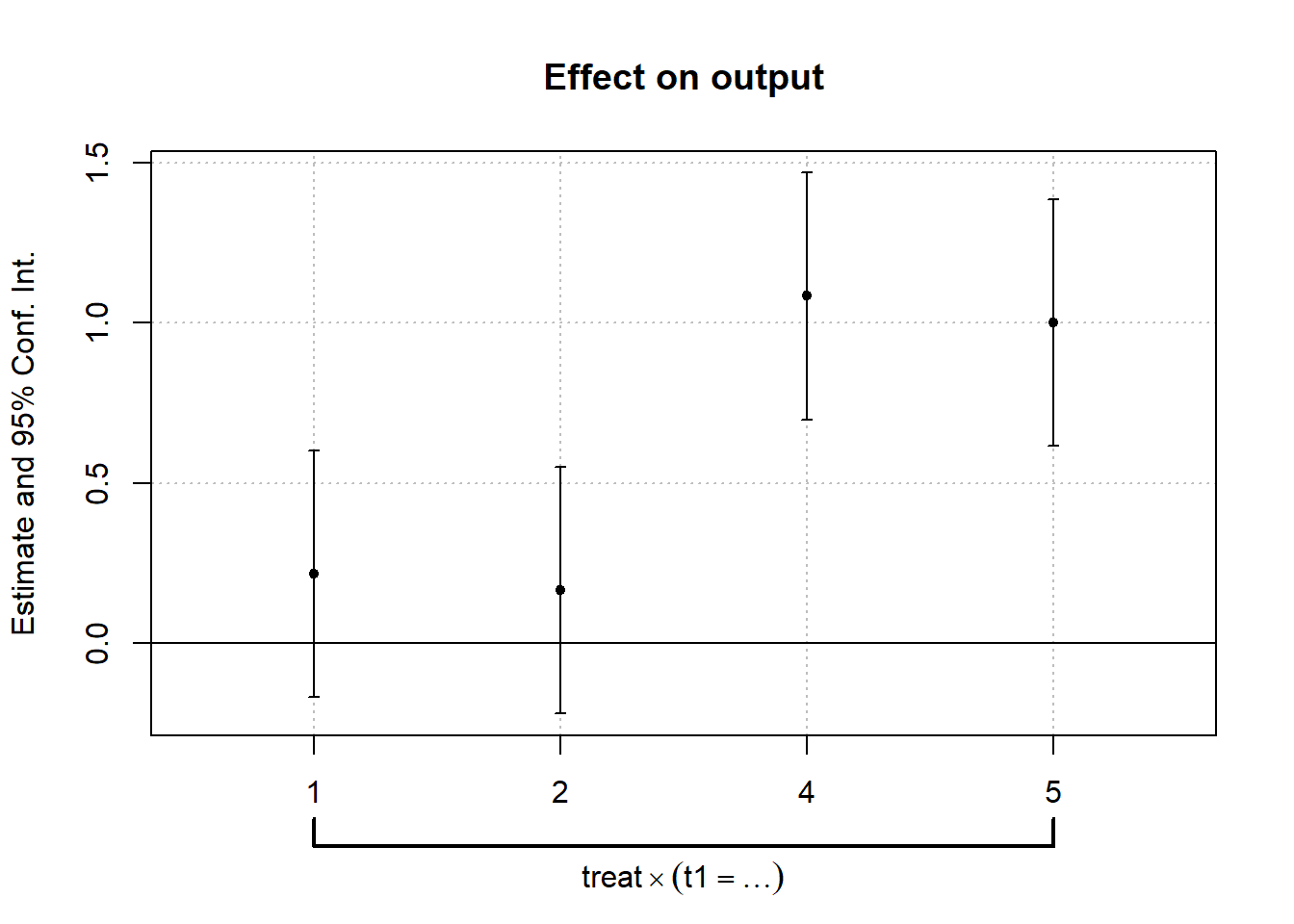
ניתן לראות שכל אחד מהאומדים בתקופת הלפני אינו שונה מאפס בצורה מובהקת.
המבחן הפורמלי יבחן ביחד את ההשערה שכל האומדים בתקופת הלפני שווים לאפס, כלומר
\[H_0=\beta_{1}=\beta_{2}=0\] \[H_1= else\]
wald(lnl,c("t1::1","t1::2")) # Equivalent to: wald(lnl,"t1::[12]:") ## Wald test, H0: joint nullity of t1::1:treat and t1::2:treat
## stat = 0.673132, p-value = 0.510296, on 2 and 1,232 DoF, VCOV: IID.אנחנו רואים שה p-value עומד על 0.51 כלומר נדחה את ההנחה שכל האומדים שווים לאפס בכל \(\alpha\) הגדול מ0.51. לא נדחה את הנחת האפס עבור ר”מ של 5%.
6.4.1.2 לאחר תיקון סטיות התקן
כעת נחזור על מבחן ה- parallel trend אבל ניקח בחשבון שהטעויות אינן בלתי תלויות זו בזו.
בפרט, נבדוק את ההשערה תחת ההנחה שהטעויות מתואמות בתוך הנבדקים.
ניתן להריץ מחדש, כאשר אנחנו משנים את פרמטר
vcov
בפונקצית האמידה, או להוסיף אותו בפונק’ הבאות
lnl.cl<-feols(output~i(t1,treat,3)|id+t1,vcov=~id,data=dt)
coefplot(lnl.cl)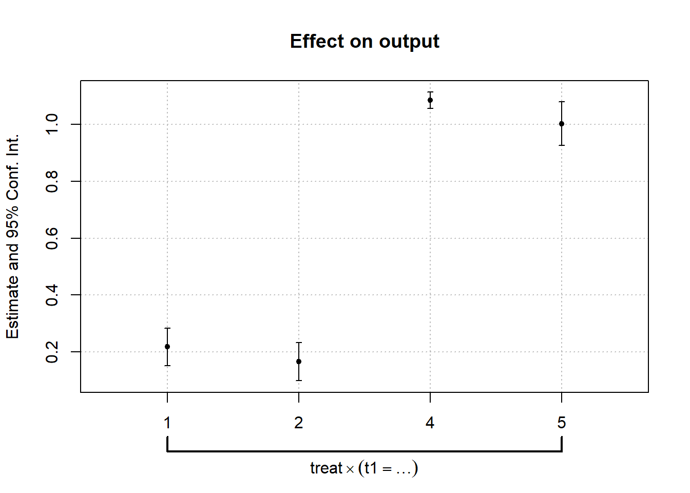
wald(lnl.cl,c("t1::1","t1::2")) # Equivalent to: wald(lnl,"t1::[12]:") ## Wald test, H0: joint nullity of t1::1:treat and t1::2:treat
## stat = 33.8, p-value = 5.035e-15, on 2 and 1,232 DoF, VCOV: Clustered (id).coefplot(lnl,vcov=~id)
wald(lnl,vcov=~id,c("t1::1","t1::2")) # Equivalent to: wald(lnl,"t1::[12]:") ## Wald test, H0: joint nullity of t1::1:treat and t1::2:treat
## stat = 33.8, p-value = 5.035e-15, on 2 and 1,232 DoF, VCOV: Clustered (id).6.5 להוסיף
6.5.1 רגרסיה לוגיסטית ופרוביט
6.5.2 רגרסייה לפי רבעונים
6.5.3 אמידה בשני שלבים ומשתני עזר
6.5.4 נתוני פאנל
library(lme4)
library(plm)
6.5.4.1 אפקט רנדומלי
6.5.4.2 אפקט קבוע
6.5.5 סדרות עתיות
6.5.5.1 סדרות הפרשים
6.5.5.2 מבחני סדרות עתיות
6.5.6 כלי עזר
6.5.6.1 Biglm
כשאנחנו עובדים עם מסד נתונים גדולים, הרצת הרגרסייה עשויה לקחת זמן,
אחת החבילות שמנסות להתמודד עם זה היא
biglm
, אופן העבודה שלה היא הרצת רגרסייה על חלק קטן מהדאטה בכל פעם ועדכון הדאטה בשלבים
(צ’אנקים)
#install.packages("biglm")
library(biglm)
data(trees)
# Random 0,1,2 number- I replaced manually the zeros from the second row- will be the 2nd chunk.
trees$type<-c(2, 0, 0, 0, 2, 1, 2, 0, 1, 1,
       2, 2,1 ,2 ,2 ,1, 1, 1, 1, 2, # row without zeros
       1, 0, 0,1, 0, 0, 0, 2, 0, 1, 1)
chunk1<-trees[1:10,]
chunk2<-trees[11:20,]
chunk3<-trees[21:31,]
כיוון שאין סוג מסויים של עצים בצ’אנק השני, הרצת קטע הקוד תוביל לשגיאה:
ff<-log(Volume)~log(Girth)+log(Height)+factor(type)
a <- biglm(ff,chunk1)
a <- update(a,chunk2)
## Error in update.biglm(a, chunk2): model matrices incompatibleהפתרון יהיה להגדיר את סוג העצים כמשתנה קטגוריאלי כבר בדאטה עצמו והרצת הרגרסייה ללא שימוש בפקטור
trees$type<-as.factor(trees$type)
chunk1<-trees[1:10,]
chunk2<-trees[11:20,]
chunk3<-trees[21:31,]

ff<-log(Volume)~log(Girth)+log(Height)+type
b <- biglm(ff,chunk1)
b <- update(b,chunk2)
b <- update(b,chunk3)
נשווה את תוצאות האמידה לרגרסייה בפקודת lm
c<-lm(log(Volume)~log(Girth)+log(Height)+factor(type),data = trees)
rbind(coef(b),coef(c))
## (Intercept) log(Girth) log(Height) type1 type2
## [1,] -6.883913 1.979145 1.180558 -0.03070903 -0.004641656
## [2,] -6.883913 1.979145 1.180558 -0.03070903 -0.004641656